Two dimensional smoothing via an optimised Whittaker smoother

Abstract

Background

In many applications where moderate to large datasets are used, plotting relationships between pairs of variables can be problematic. A large number of observations will produce a scatter-plot which is difficult to investigate due to a high concentration of points on a simple graph.

In this article we review the Whittaker smoother for enhancing scatter-plots and smoothing data in two dimensions. To optimise the behaviour of the smoother an algorithm is introduced, which is easy to programme and computationally efficient.

Results

The methods are illustrated using a simple dataset and simulations in two dimensions. Additionally, a noisy mammography is analysed. When smoothing scatterplots the Whittaker smoother is a valuable tool that produces enhanced images that are not distorted by the large number of points. The methods is also useful for sharpening patterns or removing noise in distorted images.

Conclusion

The Whittaker smoother can be a valuable tool in producing better visualisations of big data or filter distorted images. The suggested optimisation method is easy to programme and can be applied with low computational cost.

Background

The histogram -in all its simplicity- is one of the most powerful tools of data visualization. Plotting the values of a variable x against a variable y will reveal whether there are is some sort of correlation between the variables or not, whether the relationship is linear or more complicated, whether there are interesting subgroups in the data or whether outliers are present. A problem might rise however, when trying to plot many points onto one simple graph. As the number of observations becomes larger and larger many scatter-plots end up being to busy for the eye to understand. Often, in moderate to large datasets, a collection of many observations on one plane will end up revealing a cloud of points where all structure remains obscured by the superposition of one point onto another. Depending on what is the medium where such a graph will be illustrated, it becomes a waste of ink or space.

To address this problem, some researchers have suggested smoothing data to obtain a heat plot image, rather than the original scatter plot. A heat plot will use colour, or shades of black, to represent areas of great concentration of points. A common way is via the use of Kernel smoothers [1], employed in R with the function smoothScatter which is part of the base distribution [2]. More recently, Eilers and Goeman [3] illustrated a way of smoothing scatter-plots in two directions using penalized b-splines or p-splines. This approach has been implemented in package gamlss.util via command scattersmooth [4].

In this work we are focusing on the paper by Eilers and Goeman [3] where a scatter-plot is enhanced using smoothed densities. We will start off with the same approach, where penalized splines are applied on the x and y directions, respectively. However, we will also go a step further and so how the optimal smoothed scatter-plot can be obtained by estimating the amount of penalty needed for each graph. We view penalized splines as random effects whose variance depends on the penalty weight. This is not a completely new approach but has only been applied to one dimension before (see [5–8]). We will revise the algorithm and extend it to apply to two dimensional smoothing.

The paper will start by illustrating a simple spline, the Whittaker smoother [9] and how this is applied in smoothing in one direction. In the next section we will introduce a simple dataset on which we will show how to obtain an optimised smoother where the penalty weight is estimated. We will then extend the method into two dimensions and show how to optimise smoothing penalties. The paper is ended with a discussion.

Implementation

The Whittaker smoother

Consider a simple scatter-plot in which the logarithm of the ratio of received light from two laser sources (given as y) is plotted against the distance travelled before the light is reflected back to its source, or range x. These particular data are produced using the Light Detection and Ranging (LIDAR) technique. The data have been used in [10] (Chapter 3) and can be downloaded from http://matt-wand.utsacademics.info/webspr/data.html.

We would like to obtain a smooth function of y given by a vector α. That means that for each observation in vector y, written as y _i with i=1,2,...,m an estimate α _i is obtained. Adding one parameter α _i for each observation y _i has the benefit of allowing the smoother to be very flexible and follow any kind of pattern the data might have. The drawback of course is that the number of parameters is as big as the number of observations which can lead to over-fitting. To control for over-fitting, a roughness penalty is imposed based on the differences of the parameters.

Let D _d be a matrix that forms differences of order d. For example, a first order difference is denoted as Δ α _i =α _i −α _i−1, while a second order difference would be Δ ² α _i =Δ(Δ α _i )=α _i −α _i−1−(α _j−1−α _j−2), with corresponding D ₁ and D ₂ matrices given by:

$$ D_1=\left[ \begin{array}{rrrr} -1 & 1 & 0 & 0\\ 0 & -1 & 1 & 0\\ 0 & 0 & -1 & 1\\ \end{array} \right]; D_2=\left[ \begin{array}{rrrrr} -1 & -2 & 1 & 0 & 0\\ 0 & 1 & -2 & 1 & 0\\ 0 & 0 & 1 & -2 & 1\\ \end{array} \right] $$

The penalized Whittaker smoother is computed by minimising the following penalised least-squares function:

$$ S= ||y-\alpha||^{2}+\lambda||D_{d}\alpha||^{2} $$

(1)

Then, to get an explicit solution for α one needs to minimise S in (1). That would lead to penalized normal equations given as:

$$ \hat{\alpha}=(I+\lambda D^{\prime} D)^{-1} y $$

(2)

where I is an identity matrix of dimension m×m. The smoothed vector $\hat {\alpha }$ depends, of course, by the choice of the penalty weight. When λ tends to zero, hardly any penalization is imposed on the estimates giving a non-smoothed curve, close to the actual values. On the other extreme, as λ tends to infinity the penalty weight dominates and it results in a straight line. Optimal values of λ should provide a smooth curve that reveals the true nature of the data whilst removing roughness and randomness. Figure 1 illustrates the raw data along with three smooth curves based on different penalty weights. For small values of λ the data are undersmoothed, while as λ increases the methods provides a smoother curve.

Fig. 1

Whittaker smoother on the LIDAR data using three different penalty weights

Penalty optimization

A common way to choose the optimal weight is to perform a search for an optimal criterion over a fine grid of λ values. The user has to define a number of distinct possible values of λ, fit a model for each one of those and then decide which one is preferred based on some sort of a loss function or a criterion. Common choices include cross-validation or Akaikes-type criteria (including Akaike Information Criterion (AIC), Akaike Information Criterion correction (AICc), Bayesian Information Criterion (BIC) etc, see [11–13]).

One popular approach is the use of Generalized Cross Validation (GCV) [14]. Define H the hat matrix as H=(I+λ D ^′ D)⁻¹ and let ed =trace(H) be the effective dimensions, given as the sum of the diagonal elements of H. Then

$$ GCV(\lambda)=\frac{\sum_{i=1}^{m} (y_{i}-\hat{\alpha_{i}})^{2}}{(m-tr(H))^{2}} $$

(3)

Here, we use an algorithm for penalty optimisation that treats the penalty weight as a parameter to be estimated from the model. A penalized likelihood can be seen through a Bayesian model framework [15], or a random effects framework [10], or an extended likelihood of a random effect parameter [16]. These different viewpoints allow for the use of an algorithm that was first suggested by [17] to estimate the variance of the random effect in a random effects model. Variations of the algorithm have also been published in [6, 7].

In the Whittaker smoother model, define $e=y-\hat {\alpha }$ and let

$$ \hat{\sigma^{2}}=\frac{e^{\prime}e}{m-ed} $$

(4)

where m and ed as before, and let

$$ \hat{\sigma_{\alpha}^{2}}=\frac{\hat{\alpha^{\prime}}D^{\prime}D\hat{\alpha}}{ed-2} $$

(5)

More details can be found in [18] (Chapter 9).

The algorithm that chooses an optimal weight then has the following steps:

• 1. For given $\hat {\sigma ^{2}}, \hat {\sigma _{\alpha }^{2}}$ find $\hat {\lambda }=\frac {\hat {\sigma ^{2}}}{\hat {\sigma _{\alpha }^{2}}}$.

• 2. Estimate vectors by: $\hat {\alpha }=(I+\hat {\lambda }D^{\prime }D)^{-1}y$

• 3. Given α update $\hat {\lambda }=\frac {\hat {\sigma ^{2}}}{\hat {\sigma _{\alpha }^{2}}}$.

• 4. Iterate until convergence.

The algorithm usually converges within a few steps. In rare cases convergence is sensitive to starting values of λ but we have found that this is rarely happening when both $\hat {\sigma ^{2}}, \hat {\sigma _{\alpha }^{2}}$ are 1.

Smoothing a two dimensional histogram

Consider a two dimensional domain x−y that is being cut into rectangles and the number of observations that lie within each rectangle been counted. For such an x−y plain a matrix R _m×n is formed that contains counts. To smooth a two-dimensional histogram based on R, one has to smooth first the columns R _∙n , that form a vector y, using the same algorithm defined before for one dimensional smoothing. That would produce a new matrix G _m×n . Then, using exactly the same procedure it is easy to smooth the columns of $G^{\prime }_{\bullet m}$, which are the rows of G _m×n . The new smoothed matrix will be the transposed of the desired outcome. This is the algorithm that was defined in [3]. There are two different penalty weights in the algorithm, λ ₁ that penalises the smooth over columns of R _m×n and λ ₂ which is used for the penalty in rows of G _m×n . In the original paper, as well as in the function scatterSmooth the penalties are not optimised, instead they are taken with the default values: λ ₁,λ ₂=1. Since this is a two step algorithm, it would be rather straightforward to optimise λ-s into both direction. In the first step, the algorithm for one dimensional smoothing can be applied to get the optimal for the columns of R _m×n and in the second step, the same algorithm will be applied to optimize λ ₂. That would result in an overall better image of the data.

Results

The LIDAR data

For the LIDAR data, the GCV criterion was first used as a reference. A fine grid of values was defined, ranging from a very small penalty weight 0.001 that would allow the estimates to vary freely, to a large penalty of 100000 that would essentially make the estimates close to zero. The optimal value was determined to be for a high value of λ=7943. Using the algorithm to optimise the penalty weight the estimated value was $\hat {\lambda }=5758$. Although the two values look different, in fact the smooth line they produce is not distinguishable, as seen from Fig. 2, where one smooth lies on top of the other.

Fig. 2

Whittaker smoother on the LIDAR data, using cross-validation and optimisation

Simulated histogram

To illustrate the methods, a simple simulation dataset was created. Let x∼N(0,1) and y=0.7∗x+0.4x ²+0.3e where e is Gaussian noise. A total of 10000 observations were created and plotted in the upper left scatter-plot in Fig. 3. The relationship between the two variables is obscured by random Gaussian noise (showing in upper right graph). The latter scatter-plot was then smoothed using first a Whittaker smoother with optimised penalties. The algorithm estimated a penalty close to zero along the columns λ ₁<0.001 and a second penalty λ ₂=4.3 along the rows. The image produced be the smoother is shown in the lower left scatter-plot. The heatmap shows areas of great concentration of points, towards the centre of the graph, and also clearly reveals the signal behind the noise. A few randomly selected points are plotted around the heatmap. In the lower right graph, the Kernel smoother (using smoothScatter in R) also reveals the true signal, however, it is more sensitive to the noise and provides a heatmap with some features of the noise still in it.

Fig. 3

Smoothing a two dimensional histogram: simulated histogram. [Upper left graph:] The true relation between x and y, [Upper right graph:] obscured by noise, [Lower left graph:] smoothed by Whittaker smoother with optimised penalties and [Lower right graph:] smoothed by Kernel smoother

Simulated image

The Whittaker smoother can also be used of any 2-dimensional smoothing. To illustrate, consider the image in Fig. 4 (upper left) in which some Gaussian noise was added to mask the patterns (upper right). The addition of Gaussian noise masks completely the previously clear patterns. The application of a Whittaker smoother without a penalty optimisation uses a default line for both weights, thus here: λ ₁=λ ₂=1. However, in this case there is a need for bigger penalties that will control the smooth in both directions. As seen in the Fig. 3 (lower right graph) the smoother does remove some noise and hints on some of the patterns but it does not reveal the true image. Instead, when the weights are optimised (here λ ₁=23.8 and λ ₂=33.4) the pattern is clearly revealed.

Fig. 4

Smoothing a two dimensional histogram: simulated image. [Upper left graph:] A simulated image [Upper right graph:] obscured by Gaussian noise, [Lower left graph:] smoothed by Whittaker smoother with optimised penalties and [Lower right graph:] smoothed by Whittaker smoother without optimisation

Filtering a noisy mammography

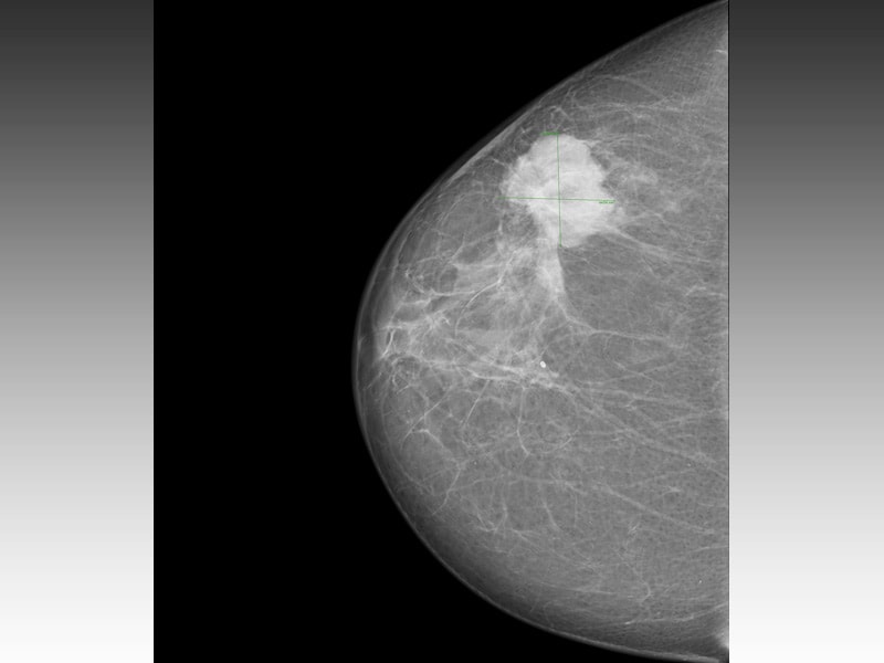
Smoothing can also be used to filter out noise from a distorted image. As an example we consider the case of a mammography. In the upper left part of Fig. 5 a mammography is displayed. In the upper part of the breast, a white shade (marked with a cross) shows signs of what might be a tumour. The original image can be found online at: http://img.medscape.com/news/2014/dt_140703_mammography_breast_cancer_800x600.jpg. To make the problem more challenging Gaussian noise has been added to the image, in a way that distorts the definition of the tumour. In Fig. 5, the original image has been slightly distorted, as it can be seen on the upper right part of the graph. To filter noise out, a kernel smoother has been used that resulted in the image shown in the lower left part of the figure. The smoother was created using function: image.smooth from library fields [19]. The smoother has removed a lot of noise and the image looks sharper, though not as sharp as the original. The Whittaker smoother was applied, with an automated selection of penalty weights. In the lower right part of the figure the Whittaker method produces a better image, has removed more noise than the kernel smoother and defined the tumour more clearly.

Fig. 5

Smoothing a two dimensional histogram: Added some noise to mammography. [Upper left graph:] A breast mammography. An area that seems like a tumour has been marked with a cross. [Upper right graph:] obscured by Gaussian noise, [Lower left graph:] smoothed by kernel smoother [Lower right graph:] smoothed by Whittaker smoother with optimisation

The merit of the method can also be seen when the image is more noisy. Figure 6 presents the same mammograph, where the addition of noise now completely distorts the image (upper right). The kernel smoother fails to reveal the original features of the image. On the contrary, using a Whittaker smoother, the features of the image are restored (lower right). Although there is still noise left, it is now more clear that there is a finding in the mammography.

Fig. 6

Smoothing a two dimensional histogram: Mammography completely distorted by noise. [Upper left graph:] A breast mammography. An area that seems like a tumour has been marked with a cross. [Upper right graph:] obscured by Gaussian noise, [Lower left graph:] smoothed by Whittaker smoother with optimised penalties and [Lower right graph:] smoothed by Whittaker smoother without optimisation

Conclusions

A simple - yet powerful addition to a Whittaker smoother was presented. The addition is based on an efficient algorithm that will lead to an optimised penalty weight. Thus, the degree of smoothing that is needed can be objectively decided by the procedure rather than subjectively by the user. The methods can be applied to one or two dimensional smoothing.

The methods presented here are intended as a tool for the applied user who would like to have an effective and computationally efficient way to smooth scatter-plots or images. The approach was illustrated and compared to a Kernel smoother or a simple Whittaker smoother. When compared with the Kernel smoother the optimised Whittaker approach produced an image with less noise and closer to the true relationship between the variables. We see a two-fold advantage here; first the optimised smoother can be used as a simple data visualisation device. It will produce a plot that is visually more compelling whilst on the same hand communicating significant information on the data. As such the differences with the Kernel smoother are minimal. Another advantage however, is that the optimised smoother can be used to gain a better insight and understanding at the data, since it removes more noise than a Kernel smoother when needed. As such, the Whittaker smooth can be used as a more in-depth explanatory method for making sense out of data.

The benefits of optimising penalty weights were also illustrated further in a second example of smoothing a simulated image. Of course, an experienced researcher will probably have been able to identify the need of a larger penalty in Fig. 4 (lower right) and experiment with larger values for the penalties. That would probably led to a better image but leads to a subjective fit that depends on the used. On the other hand, one could also optimise penalty weights by minimising some sort of loss function or criterion, as illustrated in “Background” section, but this would be a computational expensive method to follow, especially in two dimensions.

When working with real mammography images, the method was able to outperform kernel smoothers. In further investigation of the same problem, Gaussian filters have been used, to blur the image and obtain better results. When specifying a Gaussian blur, the user has to specify the variance of the Gaussian distribution. With some trial and error approach, we where able to filter the noise out to a satisfactory level, but we could not outperform the Whittaker smoother (data not shown). Additionally, the filter did require tuning from the user and was not based on an automated procedure.

A merit of our approach is that it can work even in cases where smoothing is not required. When the image is not noisy, the algorithm with converge to extremely small values for the penalty weights, thus removing the effect of the penalty altogether. The more noisy the image the bigger the penalty weights will be. These are situations where the method has great advantages over other approaches.

The algorithm presented in this paper was coded in R in just a few lines of code. It is very easy however to implement it in another programming language like Matlab or Java. The appendix contains the R programme.

Availability and requirements

Operating System: Windows 7Language: R

Appendix: R code

References

Wand M. Fast computation of multivariate kernel estimators. J Comput Graph Stat. 1994; 4(4):433–45.
R Development Core Team. R: a language and environment for statistical computing. 2014. http://www.R-project.org. Accessed 2 Mar 2017.
Eilers PH, Goeman JJ. Enhancing scatterplots with smoothed densities. Bioinformatics. 2004; 20(5):623–8.
Stasinopoulos M, Rigby B, Eilers P. Gamlss.util: GAMLSS Utilities. 2015. http://CRAN.R-project.org/package=gamlss.util.. Accessed 2 Mar 2017.
Pawitan Y. In all likelihood: statistical modelling and inference using likelihood. Oxford: Oxford Science Publications; 2001.
Perperoglou A, Eilers PH. Penalized regression with individual deviance effects. Comput Stat. 2010; 25(2):341–61.
Perperoglou A. Cox models with dynamic ridge penalties on time-varying effects of the covariates. Stat Med. 2014; 33(1):170–80.
Chountasis S, Katsikis VN, Pappas D, Perperoglou A. The whittaker smoother and the moore-penrose inverse in signal reconstruction. Appl Math Sci. 2012; 6(25):1205–19.
Whittaker ET. On a new method of graduation. Proc Edinb Math Soc. 1923; 41:63–75.
Ruppert D, Wand MP, Carroll RJ. Semiparametric Regression. Cambridge: Cambridge University Press; 2003.
Akaike H. Information theory and an extension of the maximum likelihood principle. In: Selected Papers of Hirotugu Akaike. New York: Springer: 1998. p. 199–213.
Burnham KP, Anderson DR. Model selection and multimodel inference: a practical information-theoretic approach. New York: Springer; 2002.
Bhat H, Kumar N. On the derivation of the bayesian information criterion. Merced: School of Natural Sciences, University of California; 2010.
Craven P, Wahba G. Smoothing noisy data with spline functions. Numer Math. 1978; 31(4):377–403.
Lambert P, Eilers PH. Bayesian proportional hazards model with time-varying regression coefficients: a penalized poisson regression approach. Stat Med. 2005; 24(24):3977–89.
Lee Y, Nelder JA. Hierarhical generalized linear models: a synthesis of generalized linear models, random effects models and structured dispersions. Biometrika. 2001; 88(4):987–1006.
Schall R. Estimation in generalized linear models with random effects. Biometrika. 1991; 78(4):719–27.
Lee Y, Nelder JA, Pawitan Y. Generalized linear Models with random effects: unified analysis via h-likelihood. Florida: CRC Press; 2006.
Douglas Nychka, Reinhard Furrer, John Paige, Stephan Sain. fields: Tools for spatial data Boulder, CO, USA R package version 8.4-1. 2015. doi:10.5065/D6W957CT; http://www.image.ucar.edu/fields. Accessed 2 Mar 2017.
Acknowledgements
This research has been supported by the Institute of Analytics and Data Science (IADS) funded by EPSRC. We thank the referees and the editor for valuable comments which improved the paper considerably. The first author would like acknowledge the support of UIN Sunan Kalijaga, Yogyakarta, Indonesia which sent the first author to do doctoral study.
Funding
This paper is a part of PhD research Project of the first author sponsored by The Ministry of Religious Affairs of the Republic of Indonesia. Aris Perperoglou is an academic expert in the Institute of Analytics and Data Science partly sponsored by EPSRC.
Availability of data and materials
Lidar dataset can be accessed from R-package SemiPar.
Authors’ contributions
SUZ and AP developed the formulas for estimation and conducted the simulations using R. AP conceived the original idea. Both authors read and approved the final manuscript.
Competing interests
The authors declare that they have no competing interests.
Consent for publication
Not applicable.
Ethics Approval and Consent to Participate
Author information
Authors and Affiliations
Corresponding author
Rights and permissions
Open Access This article is distributed under the terms of the Creative Commons Attribution 4.0 International License (http://creativecommons.org/licenses/by/4.0/), which permits unrestricted use, distribution, and reproduction in any medium, provided you give appropriate credit to the original author(s) and the source, provide a link to the Creative Commons license, and indicate if changes were made. The Creative Commons Public Domain Dedication waiver (http://creativecommons.org/publicdomain/zero/1.0/) applies to the data made available in this article, unless otherwise stated.
About this article
Cite this article
Zuliana, S.U., Perperoglou, A. Two dimensional smoothing via an optimised Whittaker smoother. Big Data Anal 2, 6 (2017). https://doi.org/10.1186/s41044-017-0021-9
Received:
Accepted:
Published:
DOI: https://doi.org/10.1186/s41044-017-0021-9