Evaluating associative classification algorithms for Big Data

Abstract

Background

Associative Classification, a combination of two important and different fields (classification and association rule mining), aims at building accurate and interpretable classifiers by means of association rules. A major problem in this field is that existing proposals do not scale well when Big Data are considered. In this regard, the aim of this work is to propose adaptations of well-known associative classification algorithms (CBA and CPAR) by considering different Big Data platforms (Spark and Flink).

Results

An experimental study has been performed on 40 datasets (30 classical datasets and 10 Big Data datasets). Classical data have been used to find which algorithms perform better sequentially. Big Data dataset have been used to prove the scalability of Big Data proposals. Results have been analyzed by means of non-parametric tests. Results proved that CBA-Spark and CBA-Flink obtained interpretable classifiers but it was more time consuming than CPAR-Spark or CPAR-Flink. In this study, it was demonstrated that the proposals were able to run on Big Data (file sizes up to 200 GBytes). The analysis of different quality metrics revealed that no statistical difference can be found for these two approaches. Finally, three different metrics (speed-up, scale-up and size-up) have also been analyzed to demonstrate that the proposals scale really well on Big Data.

Conclusions

The experimental study has revealed that sequential algorithms cannot be used on large quantities of data and approaches such as CBA-Spark, CBA-Flink, CPAR-Spark or CPAR-Flink are required. CBA has proved to be very useful when the main goal is to obtain highly interpretable results. However, when the runtime has to be minimized CPAR should be used. No statistical difference could be found between the two proposals in terms of quality of the results except for the interpretability of the final classifiers, CBA being statistically better than CPAR.

Introduction

Classification set of rules to form an accurate classifier [1], ARM aims at describing a dataset by means of reliable associations among patterns [2]. Associative Classification (AC) [3] come into being as the combination of the two previous fields as a way of building an interpretable and accurate classifier by means of association rules [4].

When building accurate classifiers, many different techniques have been proposed in literature such as those based on rules [5], decision trees [1] or support vector machine [6], to list a few. Many of these techniques achieve great results, but just some of them are able to build interpretable classifiers which are essential in many fields as health-care [7] or biology [8]. In general, those approaches based on rules or trees are able to obtain highly interpretable models. However, decision trees suffer from a problem of adaptability since a small change in the input data may produce large changes in the model [5]. Other approaches do not consider the whole dataset to mine rules but small samples of data and, therefore, the final classifier could not be representative of the overall trends [9]. Unlike these approaches, in AC the training phase is about searching for hidden knowledge by means of association rule mining algorithms and then a classification model (classifier) is constructed after sorting the knowledge in regards to certain criteria as well as pruning useless and redundant knowledge [4]. AC is often capable of building robust classifiers since it obtains any association rule within the dataset that can be missed by other classification systems [10]. Moreover, the rules produced in AC are easy to understand and they even could be manually updated by the end-user, unlike neural network and probabilistic approaches, which produce classification models that are hard to understand [11].

The first algorithm proposed in the AC field is known as CBA [4]. It works in two phases and the first one generates association rules by means of an exhaustive search algorithm [2]. Then, in a second phase, it ranks the discovered rules to form the final classifier. Even when this proposal obtains very interpretable and accurate classifiers, it has some problems since the runtime could take more than expected or some minority classes could be ignored. Aiming at solving these drawbacks, the same authors proposed CBA2 [12] as an improvement of the previous proposal to avoid ignoring the minority class by using multiple class minimum support. Other approaches like CMAR [12] try to solve the same problem by considering multiple rules to predict unseen examples as well as speeding up the runtime by means of complex data structures. Even all these proposals work pretty well in terms of both accuracy and efficiency, CPAR [13] was proposed as a combination of classic approaches of rule induction with features of AC obtaining both an improvement on accuracy and runtime ignoring, in part, the interpretability.

As it is described, interesting AC algorithms have been proposed in literature, obtaining good results in interpretability, predictive power and efficiency. However, with the recent need for dealing with bigger amounts of data, these proposals are becoming insufficient. Big Data is a new buzzword used to refer to the techniques used to face up the problems arising from the management and analysis of these huge quantities of data [14]. Applying existing AC approaches on such high dimensional datasets produce some limitations in terms of both computational complexity and memory requirements [15]. Hence, it is vital to propose new approaches able to scaled out [16] and to obtain results, in a reasonable quantum of time, when they are applied to Big Data.

At this point, the goal of this work is to propose two different methods based on traditional algorithms for AC (CBA and CPAR) through emerging paradigms of distributed computing (Spark and Flink). In this regard, CBA and CPAR were selected since, according to some authors [4, 12, 13, 17], these are the most interesting ones based on accuracy and interpretability. CBA is considered as the algorithm that obtains the most interpretable classifiers, whereas CPAR is able to obtain very accurate classifiers with accuracy values, in average, greater than those obtained by CBA [13]. In the experimental stage, these two proposals have been compared to existing AC approaches to demonstrate that both are the most interesting ones. In this work, the two proposed methods have been designed on both Apache Spark and Apache Flink, and these two platforms were selected since they are the most representative within the Big Data field [18]. Then, these two approaches have been compared to current state-of-art of associative classification in Big Data. It should be noted that the two proposals, that is, CBA (based on Spark and Flink) and CPAR (based on Spark and Flink), return exactly the same results as their sequential versions (CBA [4] and CPAR [13]) and the main difference lies in the runtime and the ability to be run on Big Data. The two proposals have been analyzed on 40 different datasets (30 classical datasets and 10 Big Data datasets), proving that they scale well even for file sizes up to 200 GBytes. Classical datasets were considered to find the algorithm or algorithms that best perform among sequential approaches. Such best algorithms were parallelized using Apache Spark and Flink, and considering 10 well-known Big Data datasets. Additionally, in order to prove the scalability of Big Data approaches three well-known metrics (scale-up, speed-up and size-up) have been considered to analyze how the algorithms behave on different number of nodes and data sizes [19]. Finally, it is important to remark that all the experimental results have been validated by non-parametric statistical tests.

The rest of the paper is organized as follows. “Methods” section presents the most relevant definitions and related work; “Results” section describes the proposed algorithm; “Discussion” section presents the datasets used in the experiments and the results; finally, some concluding remarks are outlined in “Conclusion” section.

Preliminaries

In this section, the associative classification task is first introduced in a formal way. Then, different paradigms for distributed computing are described.

Associative classification

The task of associative classification (AC) was proposed as a combination of two well-known tasks in the data mining fields, namely association rule mining and classification, as a way of building a interpretable and accurate classifiers [4]. In this regard, this section formally describes these two different tasks and, finally, it formally introduce the AC problem.

Let us first introduce association rule mining (ARM) in a formal way by considering a dataset comprising a set of transactions $\mathcal {T} = \{t_{1}, t_{2},..., t_{m}\}$ and a set of items or features $\mathcal {I} = \{i_{1}, i_{2},...,i_{n}\}$. Here, each transaction t_j comprises a subset of items {i_k,...,i_l}, 1≤k, l≤n. An association rule is formally defined [2] as an implication of the form X→Y where $X \subset \mathcal {I}$, $Y \subset \mathcal {I}$, and X∩Y=∅. The meaning of an association rule is that if the antecedent X is satisfied for a specific transaction t_j, i.e. X⊂t_j, then it is highly probable that the consequent Y is also satisfied for that transaction, i.e. Y⊂t_j. The frequency of an itemset $X \subset \mathcal {I}$, denoted as support(X), is defined as the number of transactions from $\mathcal {T}$ that satisfies X⊂t_j, i.e. $|\{\forall t_{j} \in \mathcal {T}: X \subseteq t_{j} ; t_{j} \subseteq \mathcal {I}\}|$. In the same way, the support of an association rule X→Y is defined as the number of transactions from $\mathcal {T}$ that satisfies both X and Y, i.e. $|\{\forall t_{j} \in \mathcal {T}: X \subset t_{j}, Y \subset t_{j} ; t_{j} \subseteq \mathcal {I}\}|$. Additionally, the strength of implication of the rule, also known as confidence, is defined as the proportion of transactions that satisfy both X and Y among those transactions that contain only the antecedent X, i.e. confidence(X→Y)=support(X→Y)/support(X) [20].

The classification task, on the contrary, can be formally defined by considering a set of items or features $\mathcal {I} = \{i_{1}, i_{2},...,i_{n}\}$ and a variable of interest or class C including a number of values. Here, a dataset is formed as a set of transactions $\mathcal {T} = \{t_{1}, t_{2},..., t_{m}\}$ and each transaction t_j comprises a subset of items {i_k,...,i_l}, 1≤k, l≤n and a specific value for the class C. The task of classification could be formally defined as predicting the class value of a l-dimensional input vector $\mathcal {S}$ such as $\mathcal {S} = \{s_{1}, s_{2},..., s_{l}\}$ where $\forall s \in \mathcal {S} : s \subseteq \mathcal {I}$. This task of mapping a set of input variables to an output variable is done by means of functions or rules [5].

AC is an special kind of classification where rules previously discovered by ARM are used to build an accurate classifier, that is, able to predict unseen examples. Aiming at obtaining this kind of classifiers many different methodologies have been proposed [10], and most of them obtain association rules by means of exhaustive search algorithms [2]. CBA [4] and its improved version CBA2 [17] are two examples of AC algorithms that first mine association rules by means of exhaustive search algorithms. However, this is a major drawback when large datasets are required to be analysed since for a dataset comprising k single items, a total of 3^k−2^k+1+1 rules can be computed and saved in memory. To solve this issue, additional approaches, e.g. CMAR [12], have been proposed which are mainly based on novel data structures that avoid the generation of any candidate. Another example is CPAR [13], which combines the advantages of AC with traditional rule induction algorithms. While these algorithms work well for not so big datasets, they cannot be used in Big Data due to the associated complexity [21]. Under these circumstances, new forms of building this type of classifiers from a Big Data perspective is an interesting and emerging topic [22], which has not received yet the needed attention.

Big Data architectures: Apache Spark, Apache Flink and its origins

MapReduce [16] is a recent paradigm of distributed computing in which programs are composed of two main stages, map and reduce. In the map phase each mapper processes a subset of input data and produces a set of 〈k,v〉 pairs. Finally, the reducer takes this new list to produce the final values. To clarify this idea, let us analyze a social network in which it is required to know the number of friends in common that each pair of friends have. Assume that friends are stored as Person→[List of friends ]. Thus, the list of friends would be something like: A→BCD, B→ACDE, C→A B D E, D→A B C E, and E→BCD. For every friend in the list of friends, the mapper will output a 〈k, v〉 pairs, where the key k is a friend along with the person (e.g. AB). The value v will be the list of friends (e.g. BCD). The key will be sorted so that the friends are in order, causing all pairs of friends to go to the same reducer. Before we send these 〈k,v〉 pairs to the reducers, we group them by their keys and get (AB)→(A C D E)(BCD). The reduce function will simply intersect the lists of values and output the same key with the result of the intersection. For example, the previous reduce ((AB)→(A C D E)(B C D)) will output (AB):(CD) which means that friends A and B have C and D as common friends.

Hadoop [23] is the de facto standard for MapReduce applications. Even when Hadoop implements these paradigms efficiently, its major drawback is it imposes an acyclic data flow graph, and there are applications that cannot be modeled efficiently using this kind of graph such as iterative or interactive analysis [18]. Besides, MapReduce is not aware of the total pipeline of map plus reduce steps so it cannot cache intermediate data in memory for faster performance. Instead, it flushes intermediate data to disk between each step. To solve these downsides, Apache Spark has risen up for solving all the deficiencies of Hadoop, introducing an abstraction called Resilient Distributed Datasets (RDD) to store data in main memory and a new approach using micro-batch technology. Unfortunately, Spark does not support native iterations, which means that its engine does not directly handle iterative algorithms [24]. In order to implement an iterative algorithm, a loop needs to repeatedly instruct Spark to execute the step function and manually check the termination criterion, significantly increasing overhead for large-scale iterative jobs. This issue is unlikely to have any practical significance on operations unless the use case requires low latency where delay of the order of milliseconds can cause significant impact. Furthermore, Flink includes its own memory manager reducing the time required by garbage collector, whereas Spark addresses this issue later with Tungsten optimization project [25]. In this sense, Apache Flink has been proposed to face the problems of Spark and to address the problem of streaming applications differently and in a more native way (vs the micro-batch methodology of Spark). By the time Flink came along, Apache Spark was already the most suitable framework for fast, in-memory Big Data analytic requirements for a number of organizations around the world. This made Flink appear superfluous, but in the recent years the attention on this new platform has risen up considerably.

Methods

In this section the two proposals are fully described. Even though the algorithms have been run on both Spark and Flink, the explanation is in common since the philosophy is the same and the unique difference is the platform. Then, In the experimental stage, these two proposals have been compared to existing AC approaches to demonstrate that both are the most interesting ones. The experimental set-up is also fully described in this section including which comparisons have been performed.

Aim of this work and our proposals

The goal of this work is to propose two different methods based on traditional algorithms for AC, that is, CBA and CPAR, through emerging paradigms of distributed computing (Spark and Flink). In this regard, CBA and CPAR were selected since, according to some authors [4, 12, 13, 17], these are the most interesting ones based on accuracy and interpretability. CBA is considered as the algorithm that obtain the most interpretable classifiers, whereas CPAR is able to obtain very accurate classifiers with accuracy values, in average, greater than those obtained by CBA [13]. In this work, the two proposed methods have been designed on both Apache Spark and Apache Flink, and these two platforms were selected since they are the most representative within the Big Data field [18].

CBA-Spark/Flink

This proposal is based on the well-known CBA [4] algorithm¹, which makes use of two different stages. Firstly, the Apriori [2] algorithm is used to find association rules. Secondly, an accurate classifier is built using the previously mined rules.

Sequential algorithm.

Aiming at easing the comprehension of the parallel approach, the original algorithm is briefly described through an example. First, association rules are extracted by means of the Apriori algorithm, only considering those rules having a support and a confidence values higher than a threshold. Let us considered the well-known weather dataset (the class attribute determines whether someone will play tennis or not) and the rules: outlook=rainy→play=no, outlook=sunny→play=yes, windy=no→play=yes, windy=noAND outlook=sunny→play=yes, windy=noAND outlook=rainy→play=no, windy=noAND outlook=rainy→play=yes. Second, an accurate classifier is built by considering the previously mined rules. In this regard, rules are sorted according to their support, confidence and size [4]. However, sorting is not enough since the final classifier might be formed of many and repetitive rules: windy=no→play=yes and windy=noAND outlook=sunny→play=yes may be fired by any example that satisfies windy=no. In this regard, the final step in the algorithm is to remove those rules with a low level of precedence and not covering at least one example on the training dataset.

Generation of association rules.

The goal of this phase is to obtain those rules whose frequency of occurrence is greater than a threshold value predefined by the user. In this sense, an iterative algorithm based on the well-known Apriori [2] is considered. An important problem of this kind of methodologies is the extremely high number of rules that may be produced at the same time. To deal with this issue, an option is not to create the whole lattice for each transaction but the l-sized sub-lattice each time, requiring a predefined number of iterations. In this regard, both the memory requirements and the computational time can be reduced. Furthermore, when the l-sized rules are generated, only the supersets from l-1-sized frequent rules are used as a seed, enabling to speed up the runtime. The explanation behind this fact is that any rule can be only frequent if all its sub-rules are also frequent [2].

This phase has been developed with a classical MapReduce application including three different types of processes: 1) driver: it is the main program when running the algorithm; 2) mappers: they aim at processing an input and producing a set of 〈k,v〉 pairs; 3) reducers: they receive the previously set of pairs in order to aggregate and filter the final results. Each of these steps are fully described as follows:

• Step 1. The driver reads the database from disk and save it in the main memory of the cluster. Either using Spark or Flink, the driver splits the dataset in data subsets in order to ease both the data access and data storage.

• Step 2. Each time this phase (see Listing 1) is performed a MapReduce procedure is run. The proposed model works by running a different mapper for each specific sub-database and, then, the results are collected and filtered in a reducer phase. These two sub-steps are described as follows.

  • Step 2.1. Mappers phase. Each mapper is responsible for mining the complete set of rules of size l for its sub-database. A set of 〈k,v〉 pairs are produced where k represents a set of items and class values, whereas v denotes an array of values (support of antecedent, support for each class value, and support of the rule considering each possible class value). All the rules produced in this step do not have any sub-set of infrequent itemsets, since the l-1-itemsets are used to avoid infrequent patterns to be generated (see Listing 1, line 3 in mapper function).

  • Step 2.2 Reducers phase. The rules for each data subsets are collected, aggregated in order to obtain the support value for the whole dataset (see Listing 1, lines 2 to 4 in reducer function), and filtered (see Listing 1, line 5 in reducer function) according to a minimum threshold for their support.

• Step 3. After the MapReduce phase is carried out, the best rules of size l are reported to the driver.

It should be noted that all these steps are repeated until l is equal to the number of the items in data. These l-sized rules are kept in a pool of rules, known as R, which will be used in the next phase, that is, the generation of the final classifier.

Building the final classifier.

The goal of this phase is to build the final classifier by means of the previously obtained rules. Let R be the set of generated rules and D the training dataset. The basic idea is to choose a set of high accurate rules from R to cover D. The final classifier is therefore formed as a list [r₁,r₂,...,r_n,default_class] where r_i∈R and default_class is only used when none of the rules is fired. This phase is tough since a huge number of combinations are possible so a heuristic is usually used to alleviate this problem.

Four different steps are considered to build the final classifier:

• Step 1. Rules are sorted according to a precedence criterion. Given two rules, r_i and r_j, r_i has a higher precedence than r_j:

  • The confidence of r_i is greater than that of r_j.

  • The confidence values are the same for both rules but the support of r_i is greater than that of r_j.

  • The confidence and support values for both rules are the same, but r_i was first generated, that is, size(r_i)<size(r_j) where size returns the number of attributes in each rule.

• Step 2. After sorting, a MapReduce is required to select candidate rules.

  • Step 2.1. Mappers phase. The input of the mappers is a chunk of the dataset and R. The goal is to iterate on each instance of the dataset to find the rule with the highest precedence that it will be fired given that example (see Listing 2). In order to do so, for each instance two rules are selected: 1)cRule: the rule with the highest precedence that correctly classify the instance; 2)wRule: the rule with also the highest precedence that wrongly classify the instance. When cRule has a higher precedence than wRule is trivial that cRule will be fired, thus it will classify this instance. However, when the contrary happens the problem is more complex and more analysis is required (these rules will be re-studied in the next step of the algorithm). When all the instances for the chunk are processed two kind of 〈k,v〉 pairs are generated:

    1)cRule type. For those rules which were selected at least one time as cRule a 〈k,v〉 pair is emitted, where k is the rule and v is an array containing two values: QFlag if it had at least one time more precedence than its wRule; classCasesCovered an array containing the number of cases per classes which were covered by this rule.

    2)wRule type. For those rules which were selected at least one time as wRule and they had a higher precedence than its respective cRule a 〈k,v〉 pair is emitted, where k is the rule and v is an array containing three values: Instance, cRule and wRule.

  • Step 2.2. Reducers phase. They receives the two types of 〈k,[v₀,...,v_n]〉 pairs generated in the previous step. In function of the type an action is done:

    1)cRule type: they are sent directly to driver, without performing any action. They are saved in the driver as Q.

    2)wRule type. The overall count is calculated aggregating the results for each mapper. In case of properties as classCasesCovered the values are added and for binary values, the OR operator is applied. Then, they are sent to the driver saving it in A.

• Step 3. Next, those complex cases which could not be studied in the previous step, are now examined. In this regard, for each case where wRule has a higher precedence than cRule is checked if this very wRule has been used as cRule for other instances (that is, QFlag is enabled) in that case is clear that wRule will cover this instance. For the another case, it is required to find all the rules with higher precedence than cRule and they also have to wrongly classify this instance. These returned rules are those that may replace cRule to cover this instance because they have higher precedences, thus in this sense the counter of covered classes are updated and they are saved. As these rules are candidate of being in the final classifier.

• Step 4. All the previously generated rules are sorted in function of the precedence of the rules. Then, all the rules which do not cover at least one instance are removed. Finally, add one by one those rules to the final classifier until the point where adding a new rule does not improve the overall performance but they worsen.

Finally, the computational complexity of this algorithm is the same as the original approach [4]. As it could be appreciated, this algorithm is computationally expensive since it is based on Apriori [2]. Let us consider N as the number of input transactions, M is the threshold and k the number of unique elements. To generate rules of size i it requires $\mathcal {O}\left (k^{i}\right)$, and for calculating support it requires $\mathcal {O}(N)$. Therefore, time complexity for algorithm would be $\mathcal {O}\left [(k+N) + \left (k^{2}+N\right) +...\right ] = \mathcal {O}\left (MN + \frac {1 - k^{M}}{1-k}\right)$.

CPAR-Spark/Flink

This proposal is based on the well-known CPAR [13] algorithm, which also works in two different stages. Firstly, a greedy approach is considered in the rule generation phase, which is much more efficient than generating all candidate rules. Secondly, CPAR repeatedly searches for the current best rule and removes all the data records covered by the rule until there is no uncovered data record.

Sequential algorithm.

CPAR² extracts rules by means of a greedy algorithm inspired in the well-known FOIL algorithm [13]. FOIL repeatedly searches for the current best rule and removes all the positive examples covered by such rule until all the positive examples in data are covered. To facilitate understanding let suppose the well-known weather dataset, where the rule with a highest gain is outlook=sunny→play=yes. Then, two items windy=no and temperature=hot are found to have similar gain. The rules outlook=sunnyAND windy=no→play=yes and outlook=sunnyAND temperature=hot→play=yes are therefore generated. This process will be repeated until all the instances are covered. Finally, to predict an unseen example the best k rules for each class is used, with the following procedure: 1) select any rule that satisfies the example; 2) from the rules selected in step 1, take the best k rules for each class; and 3) compare the average expected accuracy of the best k rules for each class and choose the class with the highest expected accuracy as the predicted class.

Generation of association rules.

This phase is responsible for obtaining class association rules. It makes use of an adaptation of FOIL which has proved to obtain good results [13]. This algorithm makes use of a unique iteration on the dataset to build a special data structure which enables to reduce the number of times that a dataset has to be read. Then, the rules could be extracted directly using this data structure. At this point, and similarly to the other proposal (CBA-Spark/Flink), this first phase has been developed with a classical MapReduce framework by including four different types of processes: 1) driver: it is the main program when running the algorithm; 2) mappers: they aim at processing an input and producing a set of 〈k,v〉 pairs; 3) reducers: they receive the previously set of pairs in order to aggregate and filter the final results; 4) a set of association rules are produced in a greedy fashion. Each of these steps are fully described as follows:

• Step 1. The driver reads the database from disk and save it in the main memory of the cluster. Either using Spark or Flink, the driver splits the dataset in data subsets in order to ease both the data access and data storage.

• Step 2. Building a data structure to synthesize the dataset. Unlike the previous approach where an iterative approach was used, in this case a unique MapReduce phase is used. The goal is to calculate the frequency of occurrence or support value for each attribute=value combined with one value of the class, that is, itemsets of size 2 where one of the items is the class and the other is an item of the form attribute=value. Therefore, for binary classification two parallel MapReduce would be required (one for positive and another for negative). In multi-class problems the process is repeated for each class value, considering the current value as positive and the rest of values as negative. This step is split in two different sub-parts as follows.

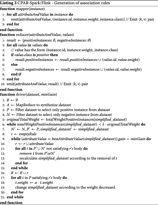
  • Step 2.1. Mapper phase (see Listing 3 mapper function). Each mapper analyzes a data subset and produces a set of 〈k,v〉 pairs where k is an expression of the form attribute=value; and v is an array of the form (instance.id, instance.weight, instance.class), where instance.id is a unique identifier for this instance; instance.weight is the weight associated to this instance (by default is 1); instance.class is the class for this instance. It should be noted that the number of mappers for this phase is limited to the size of the data, and its calculation is delegated to the platforms (Spark/Flink).

    

  • Step 2.2. Reducer phase (see Listing 3 reducer function). The set of 〈k,v〉 pairs is aggregated in the reducers to produce the final count for both the positive and negative classes of the instances for each attribute=value. Each reducer returns its result to the driver, which saves all the final results in simplified_dataset. As the number of produced 〈k,v〉 are very large a unique reducer could be act as a bottleneck. To avoid this situation, several reducers are considered to achieve a higher level of parallelism. In concrete, the meta-data (attributes and values included in data) is used to calculate the number of reducers as $numberOfReducers = \sum _{i=0}^{n} numberOfValuesForAttribute(i)$, where n is the number of attributes; numberOfValuesForAttribute(i) returns the number of different values which could take the attribute i.

• Step 3. Next, the dataset is split in subparts, one for each value of the class. It is required as a previous step of generating rules, since it will be used combined with the simplified_dataset to avoid to iterate several times in the original dataset. In case of binary classification, two new sub-sets of the original dataset would be created (see lines 3 to 4, Listing 3, driver function). Furthermore, the total weight for positive instances is calculated by the function totalWeightPositiveInstances (see line 5, Listing 3, driver function), having into account that each instance has a value of weight equal to 1 by default. In multi-class problems the problem of calculating the total weight would be repeated for each class value, iterating on the values and considering the current value as positive and the rest of values as negative.

• Step 4. Find a set of rules in a greedy fashion by means of the previously obtained data. Each rule is initialized with an empty set (see line 8, Listing 3, driver function), and the best attribute=value is selected from simplified_dataset using the gain measure. This measure is calculated as $gain(rule) = |P|\left (\log {\frac {|P*|}{|P*| + |N*| }} - \log {\frac {|P|}{|P| + |N|}}\right)$, where N and P is the number of negative instances and positive instances respectively; N∗ and P∗ are the number of both the number negative and positive instances satisfying the rule body. When the best attribute=value is selected, it is added to the current rule r (see line 10, Listing 3, driver function), then the temporal P^′, N^′ and simplified_dataset^′ are updated considering that this new rule covers some instances (see lines 11 to 14, Listing 3, driver function) and the process of adding a new attribute=value is repeated until the gain of the new attribute=value is smaller than a threshold minGain. Once the rule is completely formed, it is added to the final set of rules (see line 16, Listing 3, driver function), and P and simplified_dataset are updated considering this new rule (see lines 17 to 20, Listing 3, driver function). The process is repeated until a sufficient number of positive instances have been covered by means of the threshold δ. All the rules generated are saved in R. It generates rules while the number of positive instances in the remaining dataset are larger than a threshold (δ).

Building the final classifier

. The aim of this step is to build the final classifier by means of the previously obtained rules. Before anything, it is required to calculate the power of predictability of the rules. In this sense, the Laplace error estimate is used to calculate the accuracy of rules, which is defined as $LaplaceAccuracy = \frac {n_{c} + 1}{n_{tot} + k}$, where k is the number of classes, n_tot is the total number of examples satisfying the antecedent of the rule, among which n_c examples belong to the predicted class value c.

When an unseen example has to be predicted, the best k rules of each class are used for prediction following the next procedure. First, it selects all the rules whose antecedents are satisfied by this unseen example. Second, from the previously selected rules, it selects the best k rules for each class value. Finally, it compares the average expected accuracy of the best k rules of each class value and the class value with the highest expected accuracy is selected. Finally, it should be considered that multiple rules are used in prediction because two reasons: 1) the accuracy of rules cannot be precisely estimated; 2) it cannot be expected that any single rule can perfectly predict the class value of every example. Moreover, only the best k rules are used instead of all the rules since there are different number of rules for different class values.

Finally, the computational complexity of this algorithm is the same as the original approach [13]. During the process of building a rule, it removes in simplified_dataset each example at most once. Moreover, it takes $\mathcal {O}(k)$ time to remove an example from it. So it takes $\mathcal {O}(nk)$ time to build a rule, thus the final time complexity of calculating the ruleset is measured as $\mathcal {O}(nk|R|)$.

Experimental set-up

This section describes both the experimental set-up (algorithms and datasets) and the achieved results. The goal of this experimental analysis is four-fold:

• 1 To compare the quality of the predictions with other well-known algorithms taken from the AC field.

• 2 To analyze the interpretability of the results with regard to other methodologies.

• 3 To compare the efficiency of these approaches which obtain the best possible results in terms of both quality (accuracy and kappa) and interpretability.

• 4 To analyze the scalability in Big Data environments when different parallel implementations are considered.

All the results obtained in the experimental analysis are available at http://www.uco.es/kdis/cba-cpar/.

Design of the experimental study and criteria for selecting the best algorithms

In this analysis, 40 real-world datasets widely used by researchers in AC and Big Data datasets have been considered. Table 1 shows the number of both attributes and instances, they have been categorized into two different groups: classical datasets and Big Data datasets. All of them are publicly available at the KEEL [26] repository. For these datasets, the number of attributes ranges from 2 to 60, the number of class values varies between 2 to 23, and the number of instances ranges from 87 to 11,000,000. A 10-fold stratified cross-validation has been used, and each algorithm has been executed 5 times. Thus, the results shown for each dataset are the average results obtained from 50 different runs.

Table 1 List of datasets (in alphabetical order) used for the experimental study

Additionally, 12 different algorithms have been considered to be analyzed, which are based on different methodologies such as exhaustive search from ARM, bio-inspired methodologies, Big Data approaches as well as classic methodologies. All these algorithms, which are mainly used by researchers in the AC field, have been selected according to their efficiency and significance within the predictive tasks. It is important to note that the configurations for these algorithms are those provided by the authors in their original works. Each of these algorithms have been categorized as follows:

Classical algorithms

• CBA [4]. It is the first algorithm that was proposed in the AC field. It is based on a well-known algorithm from ARM known as Apriori [2].

• CBA2 [17]. It is an improvement of CBA that considers multiple class minimum support in rule generation.

• CMAR [12]. It uses a recognized algorithm (FP-Growth [27]) from ARM to obtain rules without candidate generation.

• CPAR [13]. It adopts a greedy algorithm to generate interval association rules directly.

• C4.5 [1]. One of the most well-known algorithms to generate a decision tree in the same way as ID3 algorithm [5].

• RIPPER [28]. It is a rule-based learner that builds a set of rules to identify the classes while minimizing the amount of error (the number of training examples misclassified by the rules).

• CORE [29]. It is a coevolutionary algorithm for rules induction. It coevolves rules and rule sets concurrently in two cooperative populations.

• OneR [30]. It is a simple, yet accurate, classification algorithm that generates one rule for each predictor in the data. Then, it selects the rule with the smallest total error as its one rule.

Big Data algorithms

• MRAC [31]. Distributed association rule-based classification scheme shaped according to the MapReduce programming model.

• MRAC+ [31]. Improved version of MRAC where some time-consuming operations were removed.

• DAC [32]. Ensemble learning which distributes the training of an associative classifier among parallel workers.

• DFAC-FFP [33]. An efficient distributed fuzzy associative classification approach based on the MapReduce paradigm.

In order to analyze each of the aforementioned algorithms, an experimental study has been performed. In this study, the main and most important criteria to choose an algorithm is described as:

• Predictive power. In this regard, accuracy rate [5] and Cohen’s kappa rate [34] have been considered. The accuracy rate (number of successful predictions relative to the total number of examples in data) has been taken since it is the most well-known metric in classification. On the contrary, an due to accuracy may achieve unfair results with imbalanced data, Cohen’s kappa rate [34] has been considered, evaluating the actual hits that can be attributed to the classifier and not by mere chance. It takes values in the range [−1,1], where a value of −1 means a total disagreement, a value of 0 may be assumed as a random classification, and a value of 1 is a total agreement. This metric is calculated as $Kappa = \frac {N{\sum }_{i=1}^{k}{x_{ii}} - {\sum }_{i=1}^{k}{x_{i\cdot }x_{\cdot i}}}{N^{2} - {\sum }_{i=1}^{k}{x_{i\cdot }x_{\cdot i}}}$, where x_ii is the count of cases in the main diagonal of the confusion matrix, N is the number of instances and, finally, x_·i and x_i· are the column and row total counts respectively.

• Interpretability has been selected as one of the main reasons of using AC, that is, to obtain interpretable classifiers that facilitate the understanding from an expert in the domain. Rules with a less quantity of attributes and classifiers formed by a small number of rules are denoted as more interpretable from a point of view of a human expert. In this sense, it is straightforward to state that the ideal classifier would be composed of a small number of rules with very few variables. Let C be a classifier including a set of rules, i.e. C={R₀,...,R_n}, the complexity or interpretability of C is calculated as $complexity(C) = n {\sum }_{i=0}^{n} attributes(R_{i})$, where n is the number of rules used by the classifier C, R_i is a specific rule of the form R_i=X→y in the position i of the classifier C, and attributes(R_i) is defined as the number of variables, i.e. |X|, that R_i includes.

• Efficiency is of great interesting since, nowadays, more and more data is daily generated and it is vital to propose approaches that are able to be scaled out and to obtain results, in a reasonable quantum of time.

Then, the analysis is exclusively focused on Big Data algorithms. Three well-known metrics have been used to show how our proposals behave [19]. Next, each metric is briefly described.

• Speed-up [19]: given a fixed job run on a small system, and then run on a larger system, the speed-up is measured as $speed-up(p) = \frac {T_{1}}{T_{p}}$, where p is the number of nodes, T₁ is the execution time on one node and T_p is the execution time on p nodes. It holds the problem size constant, and grows the system.

• Scale-up [19]: is defined as the ability of a N-times larger system to perform an N-times larger job in the same elapsed time as the original time. Thus, it measures the ability to growth both the system and the problem. It is defined as $scale-up(D, p) = \frac {T_{D1}}{T_{Dp}}$, where D is the dataset, T_D1 is the execution time for D on one node, T_Dp is the execution time for p×D on p nodes.

• Size-up [19]: it measures how much longer it takes on a given system, when the dataset size is p larger than the original dataset. It is defined as $size-up(D, p) = \frac {T_{p}}{T_{1}}$, where T_p is the execution time for processing p×D and T₁ is the execution time for processing data.

Finally, all the experiments have been run on a HPC cluster comprising 12 compute nodes, with two Intel E5-2620 microprocessors at 2 GHz and 24 GB DDR memory. Cluster operating system is Linux CentOS 6.3. As for the specific details of the used software, the experiments have been run on Spark 2.0.0 and Flink 1.3.0.

Results

All the algorithms studied in this work have been analyzed in function of the different criteria and considering non-parametric tests. The result for each analysis is as follows:

• Analysis of the predictive power: all the aforementioned algorithms have been analyzed according to both the accuracy and kappa quality measures. CPAR obtained the best result.

• Interpretability: from the best algorithms obtained in the previous study, an analysis of interpretability have been performed considering both number of rules and attributes. CBA obtained the best results.

• Efficiency: after the two previous analysis, the best algorithms have been compared with regard to quantity of time. CBA was the best algorithm.

Additionally, two additional analyses were performed. First, traditional approaches on traditional datasets were considered to prove the importance of parallelizing such algorithms. Second, Big Data algorithms and datasets were considered. The proposals for Big Data (CBA-Spark/Flink and CPAR-Spark/Flink) are deeply analyzed and compared to the state-of-the-art in Big Data proving that they scale very well in terms of metrics such as speed-up, scale-up and size-up.

Discussion

This section discuss the implications of the findings in context of existing research.

Comparative study on predictive power, interpretability and efficiency

The aim of this section is to analyze all the aforementioned algorithms according to three main criteria: predictive power, interpetability and efficiency. It is important to remark that the best algorithms for each criterion are the only ones used in the experimental analysis of the following criterion. Each of these three analyses are carried out from two different perspectives: classical algorithms and datasets (aiming at proving that our proposal outperforms the state-of-art even when a small quantity of data is considered); Big Data algorithms and datasets (aiming at comparing to current state-of-art in Big Data). Finally, it is important to remark that classical approaches cannot be run on Big Data datasets.

Analysis of the predictive power

The goal of this study is to analyze the quality of the solutions, in terms of Accuracy and Kappa measures, obtained by different algorithms.

Classical state-of-art

Analyzing the accuracy (see Table 2), it is obtained that CMAR and OneR obtained the worst results. This behavior is caused by the fact that OneR only uses a unique rule to predict on the whole datasets. It should be noted that in those datasets comprising a huge number of instances, a higher number of rules are required to cover all the instances. Besides, CMAR did not obtain good results since it optimizes the confidence measure in isolation, that is, it generates very specific classifiers that are not able to correctly predict unseen examples. As for CBA and its improved version CBA2, they obtained good results in terms of accuracy, being even close to the results obtained by C4.5. It should be highlighted that, among all the algorithms under study, CPAR obtained the best results for the Accuracy metric. Finally, focusing on the Kappa metric (see Table 2), very similar results were obtained, although in this case the difference between CPAR and C4.5 is not so high.

Table 2 Classical algorithms

In order to analyze whether there are any statistical difference in the previous results, several non-parametric tests have been performed. First, a Friedman test has been run on the Accuracy measure, obtaining a $X_{F}^{2}= 52.894$ with a critical value of 18.475 and a p-value =3.889⁻⁹. Therefore, it is possible to assert that there exist some kind of statistical difference among the algorithms for this measure with α=0.01. In the same way, a $X_{F}^{2}= 50.042$ with a critical value of 18.475 and a p-value =1.418⁻⁸ has been obtained for the Kappa metric, meaning that there exist some statistical differences among the algorithms for α=0.01. Next, a post-hoc test has been performed to state among which algorithms there exist any difference. In this regard, Table 3 shows the p-values for the Holland test with α=0.01. CPAR has been selected as control since it achieved the best ranking in the previous analysis. Focusing on the Accuracy measure, results of this post-hoc test (see Table 4) denoted some statistical differences with regard to CMAR, CORE and OneR. The rest of algorithm equally behaves in terms of Accuracy measure. Finally, focusing on the Kappa measure, results of this post-hoc test (see Table 4) revealed some statistical differences with regard to CMAR, CORE and OneR. To sum up, among the ten selected algorithms, five of them equally behave according to the predictive power (measured with Accuracy and Kappa metrics) and, therefore, additional criteria need to be used to select the best approach.

Table 3 Classical algorithms

Table 4 Classical algorithms

Big Data state-of-art

Table 5 shows the ranking for Big Data algorithms for accuracy measure. DAC obtained close results to those obtained by MRAC. MRAC+ was the next best algorithm, improving its original non-improved version (MRAC). DFAC-FFP obtained also good results but not as good as those obtained by CBA Spark/Flink. CPAR Spark/Flink has been the algorithm which achieved the best performance on accuracy measure. Similarly, Table 5 shows the ranking for kappa measure. The results are very similar to those previously obtained. The unique difference was between MRAC and MRAC+ where in this case this last algorithm obtained worse performance than MRAC. Again, CPAR Spark/Flink has been the best algorithm.

Table 5 Big Data algorithms

In order to study whether there are any statistical significant difference among the results, several non-parametric tests have been considered. First, a Friedman test has been performed on accuracy measure obtaining a $X_{F}^{2}= 36.5$ with a critical value of 15.086 and a p-value =7.543⁻⁷. Hence, it is possible to state some kind of statistical significant differences among the algorithms. Likewise, a Friedman test has also been performed on kappa measure obtaining a $X_{F}^{2}= 45.371$ with a critical value of 15.086 and a p-value =1.219⁻⁸. Next, a post-hoc test has also been performed to find among which algorithms there are any kind of differences. In this sense, Table 6 shows p-values for the Holland test with α=0.01. Thus, it could be stated that there are some statistical differences with regard to MRAC, MRAC+ and DAC. Then, it has not been possible to find differences in terms of accuracy for CPAR Spark/Flink, CBA Spark/Flink and DFAC-FFP. Finally, focusing on kappa measure (see Table 6), shows statistical differences with regard to MRAC, MRAC+ and DAC.

Table 6 Big Data algorithms

Considering these results and comparing with those obtained in classical algorithms, it is found the same behavior. CPAR obtained the best performance so much in small data as in big data. CBA did not obtain very different results than those obtained by CPAR, however in average they have been a little worse.

Analysis of the interpretability

Continuing with the analysis of the interpretability, the number of attributes per rule as well as the number of rules have been analyzed.

Classical state-of-art

The average ranking for the complexity measure is shown in Table 7. CBA obtained the best results closely followed by its improved version CBA2. CPAR, C4.5 and Ripper obtained the worst results and, among them, there are not many big differences. In order to analyze these results in a statistical way, a Friedman test has been performed, obtaining a $X_{F}^{2} = 66.647$ with a critical value of 13.277 and a p-value =2.698⁻¹⁴, meaning that it exists some kind of statistical differences among the complexity of the solutions of these algorithms. Next, a post-hoc test has been performed to state among which algorithms there exist any type of differences. In this sense, Table 3 shows the p-values for the Holland test with α=0.01. Taking into account only the interpretability, the algorithm with the best ranking has been selected as control, that is, CBA. Results of this post-hoc test proved that CPAR, C4.5 and Ripper obtained statistical significant differences with regard to CBA. However, when comparing CBA and CBA2, an additional criterion is required since no statistical difference was obtained among them for the interpretability measure.

Table 7 Classical algorithms

Big Data state-of-art

Table 8 shows the average ranking for the complexity measure. CBA Spark/Flink has outperformed the rest of algorithms achieving the most interpretable classifiers. DFAC-FFP obtained better results than CPAR Spark/Flink. This results are very similar to those obtained in classical algorithms. CPAR almost always obtains a very large number of rules hampering interpretability of classifiers. Unlikely, CBA obtained almost always the best possible results since it obtained small rules (few attributes) and classifiers with a small number of rules.

Table 8 Big Data algorithms

In order to find some statistical significant differences among the results several non-parametric test have been performed. Firstly, a Friedman test has been performed obtaining a $X_{F}^{2} = 11.450$ with a critical value of 9.210 and a p-value =0.003 proving that there are some kind of differences. Then, a post-hoc test has been performed to state among which algorithms there are differences. In this way, Table 9 shows the p-values for the Holland test with α=0.01. It proves that there are differences with regard to CPAR Spark/Flink.

Table 9 Big Data algorithms

Analysis of the efficiency

Once the predictive power and the interpretability of the solutions have been analyzed, the final criteria to be considered is efficiency. In this sense, only the best algorithms until the moment have been taken into account.

Classical state-of-art

The runtime for the CBA and CBA2 algorithms were measured, and a Wilcoxon signed rank test was performed obtaining a Z-value =−2.519 with p-value =0.005. Results denoted that some statistical differences were found when comparing CBA and CBA2 with α=0.01, CBA2 obtaining the worst results. The explanation behind this fact is simple, CBA2 needs to build a classifier by means of a close adaptation of CBA. Then, it builds a decision tree method as in C4.5 and, at the same time, a Naive-Bayes method is also performed. It means that, in the best case, CBA2 requires the same time as CBA. However, in practice, this best case was rarely found since the building of the tree also consumes a quantity of time that increases the overall runtime.

Big Data state-of-art

Finally, the runtime of the two best algorithms have been studied. Time for CBA Spark/Flink has been the average obtained in the two platforms, being both very similar. In the next section, a different study is performed to prove whether exists differences between these two platforms. A Wilcoxon signed rank test has been performed obtaining a Z-value =−2.310 obtaining that classical CBA implemented on current distributed computing obtained statistically significant differences with regard to DFAC-FFP.

Conclusions achieved with this analysis on three different criteria

After performing a complete analysis based on three different criteria, next the following conclusions could be stated. Two algorithms for AC have been selected to be adapted to Big Data platforms. On the one hand, CBA has been considered since it obtained a good trade-off among predictive power, interpretability and efficiency. On the other hand, CPAR has proved to obtain very accurate classifiers in a reduced quantum of time but the interpretability of the results is not so good compared to other such as CBA and CBA2. In this regard, if the time required to produce results can be improved, it is obvious that CPAR should be used due to its good results in predictive power. On the contrary, when a high interpretability is required, CPAR is not recommended but CBA.

Very similar results have been obtained in Big Data. CPAR Spark/Flink obtained the best results in terms of performance. When interpretability is considered, CBA Spark/Flink is the winner outperforming both DFAC-FFP and CBA Spark/Flink. Finally, CBA Spark/Flink has also obtained the most efficient results.

Scalability of the different proposals in Big Data

The goal of this analysis is to study the scalability of the different proposals in Big Data. In this regard both the original and the adaptations have been run on a series of synthetic datasets. This kind of datasets has been selected due to the fact that only the runtime is analyzed because both algorithms have proved to obtain accurate and interpretable classifiers on real-world datasets. Furthermore, synthetic datasets enables to change both the number of instances and the search space easily to study the behavior when different data sizes are considered. On this matter, the datasets have been generated following a Gaussian distribution where the number of instances ranges from 1·10⁴ to 1·10⁸, with a search space ranging from 6500 to 1.04²²⁹, and file sizes up to 200 GBytes have been included.

Figure 1 shows the behavior of the selected algorithms when the number of instances changes. As it is illustrated, when the number of instances is low CBA-Sequential is more efficient than CPAR-Sequential, that is because CBA is more direct in building the classifier than the greedy algorithm used in CPAR. Neither the implementations based on Spark or Flink obtained good runtime with few instances. When the number of instances continues growing, the approaches based on Spark And Flink obtained much better performance that sequential methodologies. Finally, it should be remarked that between the implementations of Spark and Flink of each algorithm there are not many differences, Spark obtained a small better performance than Flink although it is not game-changing. Between CBA-Spark/Flink and CPAR-Spark/Flink, this last method obtained a better performance than CBA-Spark/Flink thanks to its greedy approach that in this case is more efficient than considering all the possible cases as an exhaustive search like the used in CBA-Spark/Flink does.

Fig. 1

Runtime of the different implementations of CBA and CPAR when the number of instances drastically changes

Continuing with this study, it has also been considered of high interest to analyze how the behavior of the proposals varies when the search space changes. The search space was calculated as the number of feasible rules that can be mined from data (3^k−2^k+1−1 where k is the number of items). To perform this analysis several synthetic datasets were used where the number of attributes were changed to analyze the performance on different search spaces. In this regard, Fig. 2 shows the performance, proving that the behavior is more different than in the previous analysis. It is due to the fact that CPAR-Sequential is not as affected as CBA-Sequential thanks to its greedy methodology. With a small search space, the proposals based on Spark and Flink do not obtain a good performance however when the search space increases, they begin to obtain a very good performance. Finally when the number of search spaces highly grows, CPAR-Spark/Flink obtained a good performance followed by CBA-Spark/Flink. With this large search space sequential approaches are not able to be run, requiring several hours to end.

Fig. 2

Runtime of the different implementations of CBA and CPAR when the search space drastically increases

The analysis now continues considering only Big Data approaches. In this regard, three well-known metrics have been studied [19]. Firstly, speed-up is analyzed aiming at measuring how algorithms behave when parallelism increases (without altering data size). Figures 3 and 4 show the results when the number of nodes increases from 1 to 12 with different data sizes, as it could be seen speed-up holds linear proving that performance increases linearly with the number of nodes. Then, scale-up is analyzed to see how well the proposed algorithms handle larger datasets when more nodes are available. In this case the size of the dataset is increased in direct proportion with the number of nodes in the system. Figures 5 and 6 shows that it is practically evaluated to 1 in almost the cases being linear and proving good scalability [19]. Lastly, size-up is analyzed where the number of nodes grows from 1 to 12 and the sizes of datasets from 10 GBytes to 120 GBytes (see Figs. 7 and 8). As the result shows, the size-up performance of our proposals is also very good.

Fig. 3

Speed-up for CBA Spark and Flink when the number of nodes changes. A file size of 120 GBytes has been used

Fig. 4

Speed-up for CPAR Spark and Flink when the number of nodes changes. A file size of 120 GBytes has been used

Fig. 5

Scale-up for CBA Spark and Flink when the number of nodes changes. A file size of 120 GBytes has been used

Fig. 6

Scale-up for CPAR Spark and Flink when the number of nodes changes. A file size of 120 GBytes has been used

Fig. 7

Size-up for CBA Spark when the number of nodes changes. Only Spark version has been run on this case since it behaves in the same way as Flink

Fig. 8

Size-up for CPAR Spark when the number of nodes changes. Only Spark version has been run on this case since it behaves in the same way as Flink

Conclusion

In this work an experimental study including 40 datasets and 12 different algorithms have been performed. This analysis has been arranged having into account three different criteria. First, predictive power of the algorithms have been measured by means of both kappa and accuracy. Second, the interpretability of the classifiers have been studied. Finally, the efficiency has been also measured. After performing this experimental study, two different algorithms of the state-of-art have been selected. On the one hand, CBA has been selected since it obtained a very good predictive power, and the best results in terms of interpretability. On the other hand, CPAR was selected after obtaining the very best results for predictive power in a reduced quantum of time.

These two algorithms have been adapted to be run on Big Data platforms considering both Apache Spark and Apache Flink. These adaptations obtained the same results as the sequential approaches but in a reduced quantum of time. Finally, an analysis of the scalability has also been performed considering files sizes up to 200 GBytes proving that our methods are able to work in an efficient way in Big Data, where sequential approaches would never be able to work in a efficient way.

References

Quinlan R. C4.5: Programs for Machine Learning. San Mateo, CA: Morgan Kaufmann Publishers; 1993.
Agrawal R, Imieliński T, Swami A. Mining association rules between sets of items in large databases. SIGMOD Rec. 1993; 22(2):207–16.
Ventura S, Luna JM. Supervised Descriptive Pattern Mining; 2018.
Liu B, Hsu W, Ma Y. Integrating classification and association rule mining. In: 4th International Conference on Knowledge Discovery and Data Mining(KDD98): 1998. p. 80–6.
Han J. Data Mining: Concepts and Techniques. San Francisco, CA, USA: Morgan Kaufmann Publishers Inc.; 2011.
Cortes C, Vapnik V. Support vector networks. Mach Learn. 1995; 20:273–97.
Valdes G, Luna J, Eaton E, B Simone C, H Ungar L, D Solberg T. Mediboost: A patient stratification tool for interpretable decision making in the era of precision medicine. In scientific reports. 2016; 6:37854.
Kim SG, Theera-Ampornpunt N, Fang C-H, Harwani M, Grama A, Chaterji S. Opening up the blackbox: an interpretable deep neural network-based classifier for cell-type specific enhancer predictions. BMC Syst Biol. 2016; 10(2):54. https://doi.org/10.1186/s12918-016-0302-3.
Clark P, Niblett T. The cn2 induction algorithm. Mach Learn J. 1989; 3(4):261–83.
Thabtah FA. A review of associative classification mining. Knowl Eng Rev. 2007; 22(1):37–65.
Fong RC, Vedaldi A. Interpretable explanations of black boxes by meaningful perturbation. In: IEEE International Conference on Computer Vision, ICCV 2017, Venice, Italy, October 22-29, 2017: 2017. p. 3449–57. https://doi.org/10.1109/ICCV.2017.371.
Li W, Han J, Pei J. Cmar: Accurate and efficient classification based on multiple class-association rules. In: 2001 IEEE International Conference on Data Mining(ICDM01): 2001. p. 369–76.
Yin X, Han J. Cpar: Classification based on predictive association rules. In: 3rd SIAM International Conference on Data Mining(SDM03): 2003. p. 331–5.
Gumbus A, Grodzinsky F. Era of big data: Danger of descrimination. SIGCAS Comput Soc. 2016; 45(3):118–25. https://doi.org/10.1145/2874239.2874256.
Wu X, Zhu X, Wu GQ, Ding W. Data mining with big data. IEEE Trans Knowl Data Eng. 2014; 26(1):97–107. https://doi.org/10.1109/TKDE.2013.109.
Dean J, Ghemawat S. MapReduce: Simplified Data Processing on Large Clusters. Commun ACM - 50th Anniversary Issue: 1958 - 2008. 2008; 51(1):107–13.
Liu B, Ma Y, Wong C-K. In: Grossman RL, Kamath C, Kegelmeyer P, Kumar V, Namburu RR, (eds).Classification Using Association Rules: Weaknesses and Enhancements. Boston, MA: Springer; 2001, pp. 591–605.
Zaharia M, Chowdhury M, Franklin MJ, Shenker S, Stoica I. Spark: Cluster computing with working sets. In: Proceedings of the 2nd USENIX Conference on Hot Topics in Cloud Computing. HotCloud’10. Berkeley: USENIX Association: 2010.
DeWitt D, Gray J. Parallel database systems: The future of high performance database systems. Commun ACM. 1992; 35(6):85–98. https://doi.org/10.1145/129888.129894.
Ventura S, Luna JM. Pattern Mining with Evolutionary Algorithms; 2016.
Oneto L, Bisio F, Cambria E, Anguita D. Slt-based elm for big social data analysis. Cogn Comput. 2017; 9(2):259–74.
Siddique N, Adeli H. Nature inspired computing: An overview and some future directions. Cogn Comput. 2015; 7(6):706–14.
Lam C. Hadoop in Action, 1st edn. Greenwich, CT, USA: Manning Publications Co.; 2010.
Padillo F, Luna JM, Ventura S. Exhaustive search algorithms to mine subgroups on big data using apache spark. Prog Artif Intell. 2017; 6(2):145–58.
Xin R, Rose J. Project Tungsten: Bringing Apache Spark Closer to Bare Metal; 2015. https://databricks.com/blog/2015/04/28/project-tungsten-bringing-spark-closer-to-bare-metal.html.
Triguero I, González S, Moyano JM, Garcîa S, Alcalá-Fdez J, Luengo J, Fernández A, del Jesús MJ, Sánchez L, Herrera F. Keel 3.0: an open source software for multi-stage analysis in data mining. Int J Comput Intell Syst. 2017; 10(1):1238–49.
Han J, Pei J, Yin Y, Mao R. Mining frequent patterns without candidate generation: A frequent-pattern tree approach. Data Min Knowl Discov. 2004; 8(1):53–87.
Cohen WW. Fast effective rule induction. In: Machine Learning: Proceedings of the Twelfth International Conference: 1995. p. 1–10.
Tan KC, Yu Q, Ang JH. A coevolutionary algorithm for rules discovery in data mining. Int J Syst Sci. 2006; 37(12):835–64.
Holte RC. Very simple classification rules perform well on most commonly used datasets. Mach Learn. 1993; 11:63–91.
Bechini A, Marcelloni F, Segatori A. A mapreduce solution for associative classification of big data. Inf Sci. 2016; 332:33–55.
Venturini L, Baralis E, Garza P. Scaling associative classification for very large datasets. J Big Data. 2017; 4(1):44. https://doi.org/10.1186/s40537-017-0107-2.
Segatori A, Bechini A, Ducange P, Marcelloni F. A distributed fuzzy associative classifier for big data. IEEE Trans Cybern. 2018; 48(9):2656–69.
Ben-David A. Comparison of classification accuracy using cohen’s weighted kappa. Expert Syst Appl. 2008; 34(2):825–32.
Acknowledgments
Not rule mining and association rule mining (ARM) are two important and different fields in data mining. Whereas the first one has a predictive purpose by discovering a small applicable.
Funding
This research was supported by the Spanish Ministry of Economy and Competitiveness and the European Regional Development Fund, projects TIN2017-83445-P.
Availability of data and materials
All the results which have been used to obtain the tables and figures shown in this work are available at http://www.uco.es/kdis/cba-cpar/.
Author information
Authors and Affiliations
Contributions
All the authors contributed in equal parts. All authors read and approved the final manuscript.
Corresponding author
Ethics declarations
Ethics approval and consent to participate
Not applicable.
Consent for publication
Competing interests
The authors declare that they have no competing interests.
Publisher’s Note
Springer Nature remains neutral with regard to jurisdictional claims in published maps and institutional affiliations.
Rights and permissions
Open Access This article is distributed under the terms of the Creative Commons Attribution 4.0 International License(http://creativecommons.org/licenses/by/4.0/), which permits unrestricted use, distribution, and reproduction in any medium, provided you give appropriate credit to the original author(s) and the source, provide a link to the Creative Commons license, and indicate if changes were made. The Creative Commons Public Domain Dedication waiver (http://creativecommons.org/publicdomain/zero/1.0/) applies to the data made available in this article, unless otherwise stated.
About this article
Cite this article
Padillo, F., Luna, J. & Ventura, S. Evaluating associative classification algorithms for Big Data. Big Data Anal 4, 2 (2019). https://doi.org/10.1186/s41044-018-0039-7
Received:
Accepted:
Published:
DOI: https://doi.org/10.1186/s41044-018-0039-7